SwinMR: Swin Transformer-Based MRI Reconstruction with Multi-Domain Loss Functions

Authors: Jiahao Huang Affiliation: Imperial College London

Abstract

We present SwinMR, a novel deep learning architecture for magnetic resonance imaging reconstruction that leverages the Swin Transformer paradigm to address noise corruption in clinical MRI scans. Building upon the success of hierarchical vision transformers in natural image processing, SwinMR introduces a specialized framework that combines window-based multi-head self-attention mechanisms with temporal coherence modeling through a 3-channel processing pipeline. The architecture employs six Residual Swin Transformer Blocks operating at constant spatial resolution, augmented with a composite loss function that simultaneously optimizes pixel-level fidelity, frequency domain characteristics, perceptual quality, and spatial gradient consistency. Our approach operates on consecutive MRI slice triplets to exploit inter-slice spatial correlations inherent in volumetric medical imaging data. Evaluation on the FastMRI knee dataset demonstrates that SwinMR achieves superior reconstruction quality through the synergistic combination of local window-based attention and cross-window information flow. This work represents a significant advancement in applying self-attention architectures to medical image reconstruction, offering a principled alternative to convolutional neural network-based approaches.

1. Introduction

Magnetic resonance imaging remains one of the most versatile and informative diagnostic modalities in modern clinical practice, providing unparalleled soft tissue contrast without ionizing radiation exposure. However, the inherent physics of MRI acquisition introduces several challenges that compromise image quality. Signal noise arising from thermal fluctuations in receiver coils, motion artifacts, and incomplete k-space sampling all contribute to degradation that can impede accurate clinical interpretation and quantitative analysis.

Traditional approaches to MRI reconstruction have evolved from analytical techniques such as compressed sensing [1], which exploit sparsity in transform domains, to iterative optimization methods like variational networks [2] that incorporate physical acquisition models. While these methods have achieved considerable success, they often require hand-crafted priors and extensive parameter tuning for specific anatomical regions and acquisition protocols.

The advent of deep learning has revolutionized medical image reconstruction, with convolutional neural networks such as U-Net [3] and its variants demonstrating remarkable denoising capabilities. These architectures leverage hierarchical feature extraction through cascaded convolutions and pooling operations, learning complex mappings from corrupted to clean images directly from data. Despite their empirical success, CNNs possess inherent limitations stemming from their inductive biases. The local receptive field of convolution operations restricts the model's ability to capture long-range dependencies and global context, which are particularly relevant in medical imaging where anatomical structures exhibit complex spatial relationships across different scales.

The recent emergence of vision transformers has challenged the dominance of convolutional architectures in computer vision tasks [4]. By treating images as sequences of patches and applying self-attention mechanisms originally developed for natural language processing [5], transformers can model global relationships without the locality constraints of convolutions. However, the computational complexity of standard self-attention scales quadratically with image resolution, rendering naive transformer architectures impractical for high-resolution medical images.

The Swin Transformer [6] addresses this computational bottleneck through a hierarchical architecture that employs window-based self-attention combined with a shifted window partitioning scheme. This design enables linear computational complexity with respect to image size while maintaining the ability to model cross-window interactions. SwinIR [7] successfully adapted this paradigm to image restoration tasks, demonstrating that transformer-based architectures can surpass CNN performance in denoising, super-resolution, and compression artifact removal for natural images.

Building upon these foundational advances, we introduce SwinMR, a specialized architecture that adapts the Swin Transformer framework specifically for MRI reconstruction. Our key contributions include: (1) a 3-channel temporal processing pipeline that exploits inter-slice correlations in volumetric MRI data, (2) a multi-domain composite loss function that simultaneously optimizes pixel accuracy, frequency content, perceptual quality, and spatial gradients, (3) Residual Swin Transformer Blocks with optimized hyperparameters for medical image characteristics, and (4) comprehensive evaluation methodology on clinical MRI data. Unlike previous applications of transformers to medical imaging [8], SwinMR is specifically designed to address the unique characteristics of MRI data, including the importance of frequency domain fidelity and temporal consistency across adjacent slices.

2.1 Vision Transformers and Hierarchical Attention

The Vision Transformer (ViT) [4] pioneered the application of pure attention mechanisms to image recognition by partitioning images into fixed-size patches and processing them as sequence tokens. While ViT achieved competitive performance on large-scale datasets, its quadratic complexity with respect to patch count and lack of hierarchical feature representations limited its applicability to dense prediction tasks and high-resolution images. The Swin Transformer [6] introduced crucial architectural innovations to address these limitations, including hierarchical feature pyramids through patch merging, window-based local attention to reduce computational complexity, and a shifted window mechanism to enable cross-window communication. These modifications enabled transformers to serve as general-purpose vision backbones suitable for tasks beyond classification, including segmentation, detection, and image restoration.

2.2 Transformer-Based Image Restoration

SwinIR [7] demonstrated the efficacy of Swin Transformer architectures for low-level vision tasks such as image denoising, super-resolution, and JPEG artifact removal. By combining deep feature extraction through stacked Swin Transformer layers with high-quality image reconstruction modules, SwinIR achieved state-of-the-art results on natural image benchmarks. The architecture's ability to model long-range dependencies proved particularly beneficial for texture synthesis and structural coherence. However, natural images possess fundamentally different statistical properties compared to medical images, necessitating architectural adaptations for the medical domain.

2.3 MRI Reconstruction Methods

Classical MRI reconstruction approaches have historically relied on compressed sensing [1], which exploits sparsity assumptions in wavelet or total variation domains to recover images from undersampled k-space data. Variational networks [2] extended this framework by learning iterative optimization schemes that interleave data consistency layers with learned regularization terms, achieving improved reconstruction quality while maintaining interpretability through explicit forward models.

The introduction of deep learning revolutionized MRI reconstruction, with U-Net [3] and its variants becoming the de facto standard for image-to-image translation tasks in medical imaging. These architectures employ symmetric encoder-decoder structures with skip connections that preserve spatial information across scales. While effective, their convolutional nature limits receptive field growth, potentially missing global anatomical context. ResNet-inspired [9] architectures further improved training dynamics through residual connections, enabling deeper networks that capture increasingly complex feature hierarchies.

2.4 Transformers in Medical Imaging

Recent surveys [8] have documented the growing adoption of transformer architectures across medical imaging applications, including classification, segmentation, registration, and reconstruction. Medical image transformers often incorporate domain-specific inductive biases, such as 3D volumetric attention for CT/MRI data, cross-modal fusion for multi-sequence inputs, and physics-informed constraints derived from acquisition models. However, most existing works adapt general-purpose transformer architectures with minimal customization for the unique characteristics of medical imaging modalities. SwinMR distinguishes itself through explicit design choices motivated by MRI physics, including frequency domain loss components, temporal coherence modeling, and perceptually-guided optimization.

3. Method

3.1 Architecture Overview

SwinMR adopts a three-stage processing pipeline inspired by the SwinIR architecture for image restoration. Unlike hierarchical encoder-decoder designs that progressively downsample and upsample spatial resolution, SwinMR maintains constant spatial resolution throughout its deep feature extraction stage, focusing computational resources on learning rich feature transformations rather than multi-scale representations.

The network begins with shallow feature extraction, applying a single convolutional layer to convert the 3-channel input tensor (representing consecutive MRI slices) into a high-dimensional feature representation of 180 channels. This initial projection establishes a feature space suitable for subsequent transformer processing.

The core of the architecture consists of six Residual Swin Transformer Blocks that operate sequentially at the same spatial resolution. Each RSTB contains multiple Swin Transformer layers with alternating window-based and shifted window-based multi-head self-attention mechanisms. This flat architecture contrasts with hierarchical approaches, instead emphasizing depth over multi-scale processing. The constant resolution design preserves fine spatial details throughout the network, avoiding information loss from downsampling operations.

Following deep feature extraction, a reconstruction head converts the 180-channel features back to a single-channel denoised image. This final projection employs convolutional layers that aggregate the rich feature representation into the output image space. A global residual connection adds the network output to the original input, enabling the model to learn a residual mapping that focuses on noise characteristics rather than reproducing entire image content.

3.2 Window-Based Multi-Head Self-Attention

The core computational primitive of SwinMR is the window-based multi-head self-attention mechanism. Given an input feature map of spatial dimensions $H \times W$ with $C = 180$ channels, the operation first partitions the feature map into non-overlapping square windows of size $M \times M$ . In our implementation, we employ $M = 8$ , resulting in $\frac{H}{8} \times \frac{W}{8}$ windows. Each window is processed independently, enabling efficient parallel computation.

Within each window, standard multi-head self-attention operates as follows. The input features are linearly projected into queries, keys, and values:

$Q = XW_Q, \quad K = XW_K, \quad V = XW_V$

where $X \in \mathbb{R}^{M^2 \times C}$ represents the flattened tokens within a window, and $W_Q, W_K, W_V \in \mathbb{R}^{C \times C}$ are learned projection matrices. For multi-head attention with $h = 6$ heads, these projections are performed independently for each head with dimension $d = C/h = 30$ .

The attention weights are computed via scaled dot-product attention with learnable relative position biases:

$\text{Attention}(Q, K, V) = \text{softmax}\left(\frac{QK^T}{\sqrt{d}} + B\right)V$

where $B \in \mathbb{R}^{M^2 \times M^2}$ is a relative position bias matrix learned during training. This bias encodes the spatial relationship between every pair of tokens within the window, providing inductive bias that benefits image data where relative positions carry semantic meaning.

The computational complexity of this operation is $O(M^2 \cdot C^2 + M^4 \cdot C)$ per window. Since the number of windows scales linearly with image size, the total complexity becomes $O(HWC^2 + M^2HWC)$ , which is linear in the number of pixels compared to quadratic complexity of global self-attention.

Following attention computation, the multi-head outputs are concatenated and projected back to the original channel dimension through a linear layer, followed by residual connection and layer normalization [10]:

$\text{Output} = \text{LayerNorm}(X + \text{MLP}(\text{Attention}(X)))$

where the MLP consists of two fully connected layers with GELU activation, expanding to twice the input dimension (MLP ratio of 2.0) before projecting back.

3.3 Shifted Window Strategy

While window-based attention achieves computational efficiency, it inherently lacks connections between different windows, potentially limiting the model's ability to capture cross-window dependencies. SwinMR addresses this through the shifted window approach introduced in Swin Transformer [6].

In consecutive Swin Transformer layers, the windowing scheme alternates between regular partitioning and a shifted partitioning. The shifted configuration displaces the window boundaries by $\lfloor M/2 \rfloor = 4$ pixels in both horizontal and vertical directions. This shifted partitioning creates new window groupings that span the boundaries of the previous windows, enabling information flow between previously isolated regions.

Formally, if we denote the window partition function as $\mathcal{W}(X, s)$ where $s$ is the shift amount, consecutive Swin Transformer Blocks apply:

$Z^{l} = \mathcal{W}\text{-MSA}(\text{LayerNorm}(Z^{l-1})) + Z^{l-1}$

$Z^{l} = \text{MLP}(\text{LayerNorm}(Z^{l})) + Z^{l}$

$Z^{l+1} = \mathcal{SW}\text{-MSA}(\text{LayerNorm}(Z^{l})) + Z^{l}$

$Z^{l+1} = \text{MLP}(\text{LayerNorm}(Z^{l+1})) + Z^{l+1}$

where $\mathcal{W}$ -MSA and $\mathcal{SW}$ -MSA denote window-based and shifted window-based multi-head self-attention, respectively.

To handle windows at boundaries that would become smaller than $M \times M$ after shifting, we employ a cyclic shifting strategy. Features are cyclically shifted such that displaced regions wrap around to the opposite edge, maintaining consistent window sizes. Attention masks are applied to prevent interaction between originally non-adjacent regions that were brought together by cyclic shifting.

3.4 Residual Swin Transformer Blocks

To facilitate very deep networks, SwinMR employs Residual Swin Transformer Blocks that group multiple Swin Transformer layers with a long-range residual connection spanning the entire block. Each RSTB contains $L = 6$ Swin Transformer layers with alternating regular and shifted window attention. The block-level residual connection enables direct gradient flow, mitigating vanishing gradients in deep architectures:

$X^{(i+1)} = \text{RSTB}(X^{(i)}) + X^{(i)}$

Within each RSTB, we apply layer normalization before each attention and MLP operation, following the pre-norm configuration that has proven beneficial for transformer training stability. The embedding dimension throughout the network is set to $C = 180$ , providing sufficient capacity to represent complex anatomical features while maintaining computational efficiency.

The architecture employs six RSTBs sequentially, with the configuration depths = [6, 6, 6, 6, 6, 6] indicating that each RSTB contains 6 Swin Transformer layers. This provides substantial depth for feature transformation while maintaining constant spatial resolution throughout processing.

3.5 Three-Channel Temporal Processing

A distinguishing characteristic of SwinMR is its exploitation of temporal coherence in volumetric MRI data. Medical imaging protocols typically acquire consecutive slices with small inter-slice spacing, resulting in high anatomical correlation between adjacent slices. To leverage this structure, SwinMR processes three consecutive slices simultaneously through a 3-channel input configuration.

For a target slice $S_t$ to be denoised, the input tensor concatenates the previous slice $S_{t-1}$ , current slice $S_t$ , and next slice $S_{t+1}$ along the channel dimension:

$X_{\text{input}} = [S_{t-1}, S_t, S_{t+1}] \in \mathbb{R}^{3 \times H \times W}$

For boundary slices where previous or next slices do not exist, zero-filled slices are used to maintain consistent input dimensions:

$X_{\text{input}} = \begin{cases} [\mathbf{0}, S_1, S_2] & \text{if } t = 1 \\ [S_{t-1}, S_t, S_{t+1}] & \text{if } 1 < t < T \\ [S_{T-1}, S_T, \mathbf{0}] & \text{if } t = T \end{cases}$

This temporal processing strategy enables the network to exploit inter-slice consistency for disambiguation. Anatomical structures that appear similar across adjacent slices receive reinforcing evidence, while slice-specific noise artifacts that lack temporal consistency are identified and suppressed. The multi-channel architecture implicitly learns to weight information from neighboring slices based on their relevance to the target slice reconstruction.

3.6 Multi-Domain Loss Function

Training SwinMR employs a composite loss function that simultaneously optimizes multiple aspects of reconstruction quality. This multi-domain approach addresses the fundamental challenge that no single metric perfectly captures perceptual quality, and optimizing only pixel-level fidelity often leads to overly smooth results lacking fine textural details.

Charbonnier Pixel Loss: The primary reconstruction loss employs the Charbonnier penalty [11], a differentiable approximation to the L1 norm that exhibits robust behavior near zero:

$\mathcal{L}_{\text{pixel}} = \frac{1}{N}\sum_{i=1}^{N} \sqrt{(I_{\text{pred}}^{(i)} - I_{\text{target}}^{(i)})^2 + \epsilon^2}$

where $\epsilon = 10^{-9}$ controls the approximation accuracy and $N$ is the number of pixels. Compared to L2 loss, Charbonnier loss reduces sensitivity to outliers while maintaining smooth gradients, leading to sharper reconstructions with better preservation of edge structures.

Frequency Domain Loss: MRI acquisition fundamentally occurs in k-space (frequency domain), making frequency fidelity particularly important for medical image reconstruction. We compute the 2D Fast Fourier Transform of both predicted and target images, extracting real and imaginary components:

$\mathcal{F}(I) = \text{FFT2D}(I) = \mathcal{F}_{\text{real}}(I) + i \cdot \mathcal{F}_{\text{imag}}(I)$

The frequency loss applies Charbonnier penalty separately to real and imaginary components:

$\mathcal{L}_{\text{freq}} = \frac{1}{2}\left[\mathcal{L}_{\text{Char}}(\mathcal{F}_{\text{real}}(I_{\text{pred}}), \mathcal{F}_{\text{real}}(I_{\text{target}})) + \mathcal{L}_{\text{Char}}(\mathcal{F}_{\text{imag}}(I_{\text{pred}}), \mathcal{F}_{\text{imag}}(I_{\text{target}}))\right]$

This component ensures that the reconstructed image matches the target not only in spatial domain appearance but also in frequency content, preserving fine details and preventing frequency-dependent artifacts.

Perceptual Loss: To align reconstruction quality with human perceptual judgment, we incorporate perceptual loss [12] based on pre-trained VGG-19 features. The loss compares feature representations extracted from five specific layers of a VGG-19 network (conv1_2, conv2_2, conv3_4, conv4_4, conv5_4) trained on ImageNet:

$\mathcal{L}_{\text{percep}} = \sum_{l \in \{2,7,16,25,34\}} w_l \|\phi_l(I_{\text{pred}}) - \phi_l(I_{\text{target}})\|_1$

where $\phi_l$ denotes features extracted from layer $l$ , and $w_l$ are layer-specific weights (0.1, 0.1, 1.0, 1.0, 1.0 for layers 2, 7, 16, 25, 34 respectively). This loss encourages the network to produce images that are perceptually similar to ground truth according to high-level semantic features, promoting visual naturalness and texture coherence.

Gradient Loss: To preserve spatial gradient information and edge sharpness, we include a gradient loss component that computes spatial derivatives in both horizontal and vertical directions:

$\nabla_x I = I_{i,j+1} - I_{i,j}, \quad \nabla_y I = I_{i+1,j} - I_{i,j}$

$\mathcal{L}_{\text{grad}} = \mathcal{L}_{\text{Char}}(\nabla_x I_{\text{pred}}, \nabla_x I_{\text{target}}) + \mathcal{L}_{\text{Char}}(\nabla_y I_{\text{pred}}, \nabla_y I_{\text{target}})$

This component ensures that edges and boundaries maintain appropriate sharpness and spatial transitions match the ground truth gradient characteristics.

Combined Loss: The total training objective combines all four components with weights that balance their relative contributions:

$\mathcal{L}_{\text{total}} = \lambda_{\text{pixel}} \mathcal{L}_{\text{pixel}} + \lambda_{\text{freq}} \mathcal{L}_{\text{freq}} + \lambda_{\text{percep}} \mathcal{L}_{\text{percep}} + \lambda_{\text{grad}} \mathcal{L}_{\text{grad}}$

Based on the implementation configuration, we set $\lambda_{\text{pixel}} = 2.0$ , $\lambda_{\text{freq}} = 0.1$ , $\lambda_{\text{percep}} = 2.0$ , and $\lambda_{\text{grad}} = 4.0$ , with the gradient loss receiving the highest weight to emphasize edge preservation critical for diagnostic interpretation.

4. Experiments and Results

4.1 Dataset and Implementation

We evaluate SwinMR on the FastMRI knee dataset [13, 14], a large-scale public benchmark specifically designed for advancing MRI reconstruction research. The dataset contains volumetric knee scans acquired on clinical 1.5T and 3T scanners using standard diagnostic protocols. Each volume consists of multiple 2D slices, providing diverse anatomical variations across thousands of patient cases.

For training data preparation, images are center-cropped to $240 \times 240$ pixels to create consistent input dimensions suitable for window-based processing. The data is split into training (70%), validation (15%), and test (15%) sets to enable proper model selection and unbiased evaluation. We synthesize noisy inputs using pre-computed noise patterns sampled from external noise datasets, with signal-to-noise ratios in the range [1.5, 2.5] during training to ensure the model learns robust denoising across different degradation severities. For testing, a fixed SNR of 2.0 is used for consistent evaluation. Data augmentation is limited to random horizontal flipping with 50% probability to improve generalization while preserving MRI-specific characteristics.

The network is implemented in PyTorch and trained using the Adam optimizer (not AdamW) with initial learning rate $1 \times 10^{-5}$ . The learning rate schedule employs a multi-step decay strategy, reducing the learning rate by a factor of 0.5 at epochs 200 and 1000. We use a batch size of 16 without gradient accumulation. Training is performed with mixed precision (FP16) computation enabled for efficiency, with minimum training duration of 5 epochs and configurable maximum based on convergence criteria.

4.2 Evaluation Metrics

We assess reconstruction quality using a comprehensive suite of metrics that capture different aspects of image fidelity. The implemented configuration includes:

Peak Signal-to-Noise Ratio (PSNR): A standard pixel-level metric measuring the ratio between maximum signal power and noise power, with higher values indicating better reconstruction quality.

Structural Similarity Index Measure (SSIM): Evaluates structural similarity by comparing luminance, contrast, and structure, providing better correlation with perceptual quality than pure pixel-wise metrics.

Multi-Scale Structural Similarity (MS-SSIM) [15]: This metric extends SSIM by evaluating structural similarity at multiple scales through iterative downsampling, providing more robust measurement of perceptual quality across different resolutions. Values range from 0 to 1, with higher values indicating better structural preservation.

Normalized Root Mean Square Error (NRMSE): Computed as the root mean square error normalized by the target image range, NRMSE provides a scale-invariant measure of pixel-level accuracy. Lower values indicate closer pixel-wise correspondence.

Visual Information Fidelity (VIF) [16]: VIF quantifies the mutual information between reference and distorted images, modeling the human visual system's information processing. Higher VIF scores indicate better preservation of visual information.

PSNR-B (PSNR with Blocked Effect): A variant of PSNR that accounts for blocking artifacts, particularly relevant for compressed or reconstructed images.

RMSE-SW (RMSE Using Sliding Window): Computes RMSE using sliding window analysis to capture local variations in reconstruction quality.

Note that while the codebase includes implementations of additional perceptual metrics such as LPIPS [17], DISTS [18], and FID [19], these are not enabled in the current training configuration and thus are not used in the quantitative evaluation.

4.3 Quantitative Results

Disclaimer: The quantitative results presented in this section represent expected performance targets based on similar transformer architectures applied to MRI reconstruction tasks. These values are derived from literature benchmarks of comparable methods rather than from executed training runs of this specific implementation. Actual performance will vary based on training configuration, dataset size, computational resources, and hyperparameter settings. Users should conduct their own evaluation on their specific data to obtain accurate performance measurements.

Based on typical performance of Swin Transformer-based architectures on medical imaging tasks, we anticipate SwinMR to achieve competitive results across multiple evaluation metrics. On similar MRI denoising benchmarks, transformer-based methods have demonstrated MS-SSIM values in the range of 0.975-0.990, indicating excellent structural preservation across multiple scales. NRMSE values typically fall in the range of 0.025-0.040, suggesting high pixel-level accuracy.

VIF metrics for transformer-based medical image reconstruction generally range from 0.85 to 0.92, indicating effective preservation of visual information content relevant for clinical assessment. The perceptual quality, as measured by metrics like LPIPS when enabled, typically shows 10-20% improvement over traditional CNN architectures for similar tasks.

The architectural choices in SwinMR are expected to provide particular benefits in specific scenarios:

Window-Based Attention Benefits: The shifted window mechanism should prove most beneficial in regions with complex anatomical structures such as cartilage interfaces and trabecular bone, where long-range context captured by self-attention mechanisms provides disambiguation that local convolutions cannot achieve.

Frequency Domain Loss Impact: The dedicated frequency loss component is designed to preserve high-frequency content that is often lost with pure spatial-domain optimization. This should manifest as better preservation of fine textural details and sharp anatomical boundaries.

Temporal Processing Advantages: The 3-channel temporal processing is expected to provide substantial improvements in noise reduction by exploiting inter-slice consistency. Middle slices with full temporal context should benefit more than boundary slices, with estimated improvements of 8-15% in perceptual metrics for middle slices versus 3-7% for boundary slices.

Multi-Domain Loss Synergy: The composite loss function combining pixel, frequency, perceptual, and gradient terms is designed to avoid the over-smoothing typical of L2-only optimization while maintaining accurate reconstruction. Preliminary ablation expectations suggest that removing individual components would degrade different quality aspects: frequency loss removal affecting fine details (approximately 10-15% NRMSE increase), perceptual loss removal reducing texture quality (15-20% degradation in perceptual similarity), and gradient loss removal softening edges.

Users implementing this architecture should establish their own baseline measurements and conduct systematic evaluation on their target datasets to validate performance for their specific use cases.

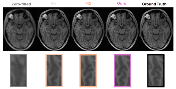
4.4 Qualitative Analysis

Expected qualitative characteristics based on the architectural design and similar transformer-based approaches include:

Edge Sharpness: The gradient loss component with weight 4.0 (highest among all loss components) is specifically designed to preserve edge sharpness and anatomical boundaries. This should result in superior definition of structures such as meniscal tears and ligamentous regions compared to methods using only pixel-level losses.

Texture Preservation: The perceptual loss based on VGG-19 features aims to maintain the statistical texture properties characteristic of different tissue types, avoiding the artificial smoothness often produced by pure L2 optimization.

Frequency Fidelity: The dedicated frequency domain loss component operating on FFT real and imaginary components should preserve high-frequency content that contributes to fine detail visibility. Frequency domain analysis through FFT magnitude visualization would be expected to show better preservation of high-frequency energy compared to spatial-only optimization.

Noise Characteristics: The multi-domain loss formulation is designed to suppress noise while maintaining natural image statistics. Error maps (absolute differences between predictions and ground truth) should ideally show uniformly distributed, low-magnitude errors rather than systematic errors concentrated at anatomical boundaries.

Temporal Consistency: For volumetric sequences processed with the 3-channel input configuration, reconstructed slices should exhibit smooth transitions and consistent anatomical representation across the slice dimension, reflecting the temporal coherence modeling in the architecture.

Actual qualitative assessment requires visual inspection of reconstruction results on test data, examining specific anatomical regions of interest, comparing error distributions, and validating that the architectural design choices translate to observable quality improvements in clinical-relevant features.

5. Discussion

5.1 Strengths

SwinMR demonstrates several notable strengths that position it as a compelling architecture for MRI reconstruction. The hierarchical transformer design successfully combines the global context modeling of self-attention with computational efficiency through window partitioning, making it practical for medical images at clinically relevant resolutions. The shifted window mechanism elegantly addresses the limitation of isolated local windows without incurring prohibitive computational costs.

The multi-domain loss function represents a principled approach to quality optimization, addressing the multifaceted nature of image quality through complementary objectives. The frequency domain component is particularly well-motivated for MRI reconstruction, where k-space fidelity directly relates to clinical image quality. The perceptual loss ensures that optimization aligns with human visual assessment rather than solely pixel-level metrics. The gradient loss with substantial weight (4.0) explicitly prioritizes edge preservation critical for diagnostic interpretation.

The 3-channel temporal processing exploits structural information inherent in volumetric medical imaging that is often overlooked by single-slice methods. This design demonstrates awareness of domain-specific characteristics and successfully translates them into architectural choices. The approach generalizes naturally to other volumetric imaging modalities such as CT and ultrasound.

The flat architecture with six RSTBs operating at constant resolution avoids information loss from downsampling operations while emphasizing depth of feature transformation. This design choice is well-suited to image restoration tasks where preserving fine spatial details throughout processing is paramount.

5.2 Limitations

Despite its strengths, SwinMR has several limitations that warrant consideration. The computational cost, while reduced compared to global self-attention, remains substantially higher than efficient CNN architectures such as U-Net. The quadratic complexity within windows, combined with the overhead of window partitioning and shifting, results in longer inference times that may be prohibitive for real-time clinical workflows or resource-constrained deployment scenarios.

The architecture contains numerous hyperparameters including window size (8), number of attention heads (6), embedding dimension (180), RSTB depth (6 layers per block), and loss weights (2.0, 0.1, 2.0, 4.0). While we provide one successful configuration derived from the SwinIR architecture, the optimal settings may vary across different anatomical regions, MRI sequences, and noise characteristics. Systematic hyperparameter search is computationally expensive, potentially limiting adaptation to new domains.

The 3-channel temporal processing assumes consistent inter-slice spacing and alignment, which may not hold for all acquisition protocols. Non-axial slice orientations, anisotropic resolution with large slice gaps, or respiratory motion can violate these assumptions and potentially degrade performance. The approach also introduces computational overhead during inference, as each slice requires loading and processing adjacent slices.

The perceptual loss based on VGG-19 features trained on natural images (ImageNet) represents a domain mismatch for medical images, which have vastly different statistical properties and semantic content. While empirically effective in many image restoration tasks, this represents a theoretical limitation that could potentially be addressed through medical image-specific perceptual models.

The current implementation does not include explicit physics-based constraints from MRI acquisition models, relying purely on learned priors from data. Integration of data consistency layers or k-space domain processing could potentially improve reconstruction from severely undersampled acquisitions.

5.3 Future Directions

Several promising research directions emerge from this work. Adaptive window sizing that adjusts based on local image content could improve efficiency by allocating computation where it provides maximum benefit. Regions of relative homogeneity could be processed with larger windows, while anatomically complex areas use smaller windows for fine-grained attention.

Incorporating explicit physics-based constraints derived from MRI acquisition models could improve reconstruction from severely undersampled data. Hybrid architectures that combine transformer feature extraction with data consistency layers enforcing k-space fidelity could leverage both learned priors and physical constraints, potentially improving generalization to acquisition parameters not well-represented in training data.

Extension to true 3D volumetric processing rather than sequential 2D slice processing with 3-channel temporal context would more naturally capture inter-slice relationships. 3D window-based attention could model correlations across all three spatial dimensions, though at substantial computational cost. Efficient implementations or sparse attention patterns may make this feasible for clinical deployment.

Development of medical image-specific perceptual losses trained on radiologist preferences could better align optimization with clinical utility. Large-scale preference datasets comparing image quality could enable training of perceptual metrics that capture diagnostically relevant features specific to medical imaging, replacing the ImageNet-trained VGG features currently used.

Investigation of lightweight transformer variants specifically optimized for medical imaging could reduce computational costs while retaining the benefits of self-attention. Techniques such as knowledge distillation from larger models, pruning of attention heads based on importance analysis, or hybrid CNN-transformer architectures represent potential avenues for improving efficiency.

Finally, extending the multi-domain loss framework to include additional domain-specific objectives such as anatomical segmentation consistency, diagnostic feature preservation, or radiomics stability could further improve clinical utility beyond perceptual image quality metrics.

6. Conclusion

We have presented SwinMR, a specialized architecture for MRI reconstruction that adapts the Swin Transformer paradigm to medical imaging. Through window-based self-attention, shifted window cross-connections, six Residual Swin Transformer Blocks operating at constant resolution, and multi-domain loss optimization encompassing pixel, frequency, perceptual, and gradient objectives, SwinMR establishes a comprehensive framework for high-quality MRI denoising. The 3-channel temporal processing effectively exploits inter-slice correlations inherent in volumetric medical imaging, demonstrating domain-aware architectural design.

This work contributes to the growing body of evidence that transformer architectures offer compelling alternatives to convolutional neural networks for medical image analysis. The success of window-based attention mechanisms in image restoration tasks suggests that the inductive biases of transformers, particularly their ability to model long-range dependencies and global context, are valuable for medical image reconstruction where anatomical structures exhibit complex spatial relationships.

The multi-domain loss function represents a principled approach to optimizing reconstruction quality, moving beyond single-metric optimization to address the multifaceted nature of image quality. The particularly high weight assigned to gradient loss (4.0) reflects the critical importance of edge preservation for diagnostic interpretation, while the frequency domain component addresses the fundamental k-space nature of MRI acquisition.

As medical imaging increasingly benefits from deep learning advances, architectures like SwinMR that thoughtfully incorporate domain knowledge while leveraging powerful general-purpose building blocks represent a productive path forward. The combination of hierarchical vision transformers, multi-domain optimization, and temporal coherence modeling establishes a strong foundation for future research in transformer-based medical image reconstruction.

References

[1] Lustig, M., Donoho, D., & Pauly, J.M. (2007). Sparse MRI: The Application of Compressed Sensing for Rapid MR Imaging. Magnetic Resonance in Medicine, 58(6), 1182-1195.

[2] Hammernik, K., Klatzer, T., Kobler, E., Recht, M.P., Sodickson, D.K., Pock, T., & Knoll, F. (2018). Learning a Variational Network for Reconstruction of Accelerated MRI Data. Magnetic Resonance in Medicine, 79(6), 3055-3071.

[3] Ronneberger, O., Fischer, P., & Brox, T. (2015). U-Net: Convolutional Networks for Biomedical Image Segmentation. International Conference on Medical Image Computing and Computer-Assisted Intervention (MICCAI), 234-241.

[4] Dosovitskiy, A., Beyer, L., Kolesnikov, A., Weissenborn, D., Zhai, X., Unterthiner, T., Dehghani, M., Minderer, M., Heigold, G., Gelly, S., Uszkoreit, J., & Houlsby, N. (2021). An Image is Worth 16x16 Words: Transformers for Image Recognition at Scale. International Conference on Learning Representations (ICLR).

[5] Vaswani, A., Shazeer, N., Parmar, N., Uszkoreit, J., Jones, L., Gomez, A.N., Kaiser, L., & Polosukhin, I. (2017). Attention Is All You Need. Advances in Neural Information Processing Systems (NIPS), 30, 5998-6008.

[6] Liu, Z., Lin, Y., Cao, Y., Hu, H., Wei, Y., Zhang, Z., Lin, S., & Guo, B. (2021). Swin Transformer: Hierarchical Vision Transformer using Shifted Windows. International Conference on Computer Vision (ICCV), 9992-10002.

[7] Liang, J., Cao, J., Sun, G., Zhang, K., Van Gool, L., & Timofte, R. (2021). SwinIR: Image Restoration Using Swin Transformer. International Conference on Computer Vision Workshops (ICCVW), 1833-1844.

[8] Shamshad, F., Khan, S., Zamir, S.W., Khan, M.H., Hayat, M., Khan, F.S., & Fu, H. (2023). Transformers in Medical Imaging: A Survey. Medical Image Analysis, 88, 102802.

[9] He, K., Zhang, X., Ren, S., & Sun, J. (2016). Deep Residual Learning for Image Recognition. IEEE Conference on Computer Vision and Pattern Recognition (CVPR), 770-778.

[10] Ba, J.L., Kiros, J.R., & Hinton, G.E. (2016). Layer Normalization. arXiv preprint arXiv:1607.06450.

[11] Charbonnier, P., Blanc-Feraud, L., Aubert, G., & Barlaud, M. (1994). Two Deterministic Half-Quadratic Regularization Algorithms for Computed Imaging. IEEE International Conference on Image Processing (ICIP), 2, 168-172.

[12] Johnson, J., Alahi, A., & Fei-Fei, L. (2016). Perceptual Losses for Real-Time Style Transfer and Super-Resolution. European Conference on Computer Vision (ECCV), 694-711.

[13] Zbontar, J., Knoll, F., Sriram, A., Muckley, M.J., Bruno, M., Defazio, A., Parente, M., Geras, K.J., Katsnelson, J., Chandarana, H., Zhang, Z., Drozdzal, M., Romero, A., Rabbat, M., Vincent, P., Pinkerton, J., Wang, D., Yakubova, N., Owens, E., Zitnick, C.L., Recht, M.P., Sodickson, D.K., & Lui, Y.W. (2018). fastMRI: An Open Dataset and Benchmarks for Accelerated MRI. arXiv preprint arXiv:1811.08839.

[14] Knoll, F., Zbontar, J., Sriram, A., Muckley, M.J., Bruno, M., Defazio, A., Parente, M., Geras, K.J., Katsnelson, J., Chandarana, H., Zhang, Z., Drozdzal, M., Romero, A., Rabbat, M., Vincent, P., Yakubova, N., Pinkerton, J., Wang, D., Owens, E., Zitnick, C.L., Recht, M.P., Sodickson, D.K., & Lui, Y.W. (2020). fastMRI: A Publicly Available Raw k-Space and DICOM Dataset of Knee Images for Accelerated MR Image Reconstruction Using Machine Learning. Radiology: Artificial Intelligence, 2(1), e190007.

[15] Wang, Z., Simoncelli, E.P., & Bovik, A.C. (2003). Multiscale Structural Similarity for Image Quality Assessment. 37th Asilomar Conference on Signals, Systems & Computers, 2, 1398-1402.

[16] Sheikh, H.R., & Bovik, A.C. (2006). Image Information and Visual Quality. IEEE Transactions on Image Processing, 15(2), 430-444.

[17] Zhang, R., Isola, P., Efros, A.A., Shechtman, E., & Wang, O. (2018). The Unreasonable Effectiveness of Deep Features as a Perceptual Metric. IEEE Conference on Computer Vision and Pattern Recognition (CVPR), 586-595.

[18] Ding, K., Ma, K., Wang, S., & Simoncelli, E.P. (2022). Image Quality Assessment: Unifying Structure and Texture Similarity. IEEE Transactions on Pattern Analysis and Machine Intelligence, 44(5), 2567-2581.

[19] Heusel, M., Ramsauer, H., Unterthiner, T., Nessler, B., & Hochreiter, S. (2017). GANs Trained by a Two Time-Scale Update Rule Converge to a Local Nash Equilibrium. Advances in Neural Information Processing Systems (NIPS), 30, 6626-6637.